Finite Element Method Simulation

Problem / Goal

Simulating the physical behavior of soft materials requires more than simple mass-spring systems. To capture realistic volume preservation and stress responses, we must model Continuum Mechanics.

The goal was to implement a robust 3D FEM solver capable of handling both small (Linear Elastic) and large (Neo-Hookean) deformations, solving for static equilibrium where internal elastic forces balance external loads.

My Contribution

I built the simulation engine from the ground up:

• Continuum Mechanics: Modeled deformation using the Deformation Gradient (F) and the First Piola-Kirchhoff stress tensor (P).
• Material Models: Implemented both Linear Elasticity (Hooke's Law) and Neo-Hookean hyperelasticity.
• Sparse Solvers: Assembled global Stiffness Matrices (K) and utilized sparse conjugate gradient solvers for efficiency.
• Nonlinear Optimization: Implemented Newton's Method with a backtracking line search to robustly solve the nonlinear energy minimization problem.

Technical Approach

1. Stiffness Matrix Assembly

A critical part of FEM is assembling the global stiffness matrix from element-wise contributions. This function computes the derivative of force with respect to position, effectively the "spring constant" for the entire mesh.

def stiffness_matrix(self, vertices: array) -> spmatrix:
    """ Computes the global sparse stiffness matrix K. """
    
    # Iterate over all tet elements
    for t in range(num_tets):
        # ... (retrieve deformation gradient F) ...

        # Compute element contribution Kt = volume * dP/dx * dF/dx
        # Chain rule: dP/dx = dP/dF * dF/dx
        vol = volumes[t]
        dP_dF = material.stress_differential(F)
        dF_dxt = dF_dx[t]

        dP_dxt = dP_dF @ dF_dxt
        Kt = vol * dF_dxt.T @ dP_dxt

        # Map local 12x12 matrix to global indices
        for i in range(m):
            for j in range(m):
                triplets.append([index_map[i], index_map[j], Kt[i, j]])

    # Construct the sparse matrix from triplets
    K = csc_matrix((vals, (row_inds, col_inds)), shape=(N*dim, N*dim))
    return K

2. Neo-Hookean Material Model

The Neo-Hookean model extends linear elasticity to handle large rotations and deformations physically correctly. It uses the logarithm of the determinant of the deformation gradient ($J$) to enforce volume preservation (resisting compression to zero volume).

class NeoHookean(Material):
    def energy_density(self, F: array) -> float:
        """
        Compute energy density W for hyperelastic material.
        W = 0.5 * mu * (I1 - dim - 2*log(J)) + 0.5 * lm * log(J)^2
        """
        dim = F.shape[0]
        I1 = np.dot(F.ravel(), F.ravel())
        logJ = np.log(np.linalg.det(F))
        W = 0.5 * self.mu * (I1 - dim - 2 * logJ) + 0.5 * self.lm * logJ ** 2
        return W

    def stress_tensor(self, F: array) -> array:
        """ First Piola-Kirchhoff stress tensor P. """
        F_invT = np.linalg.inv(F).T
        logJ = np.log(np.linalg.det(F))
        P = self.mu * (F - F_invT) + self.lm * logJ * F_invT
        return P

Validation / Results

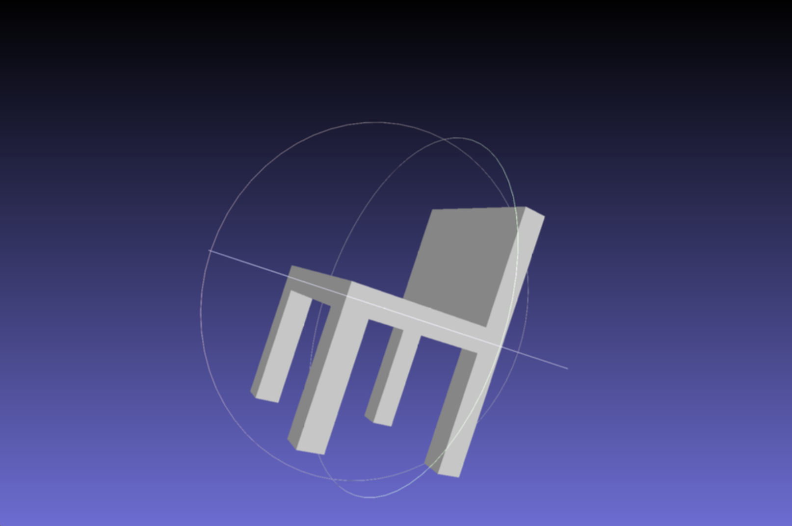
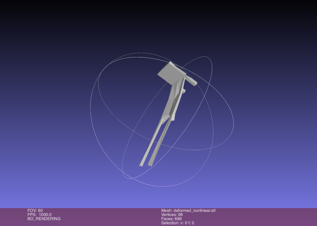
The simulation was validated by subjecting meshes to large gravity loads. The Neo-Hookean model correctly demonstrated nonlinear stiffening at high strains, unlike linear elastic models which would invert or "blow up."

Lessons + Next Steps

Lesson: Implementing standard Newton's Method is rarely enough for physics simulation. A robust line search (globalization strategy) is absolutely necessary to prevent the solver from taking steps that invert elements.

Next Steps: Extending the system to support dynamic simulation with implicit time integration (Backward Euler) for stable motion.

Links